10/10/2022

Lab 1 - Deep Neural Networks in PyTorch

#machinelearning #course #fsdl

Follow along with the Lab 1 notebook. Or check out the course website for the Lab 1 slides.

Setup

Using a bootstrap python file, the Colab environment is setup to pull the FSDL github repo and set the path variable, lab directory, hot reloading of modules, and inline plotting.

Downloading data

We will be using the mnist dataset of handwritten digits. This is downloaded as a pkl.gz serialized file from the PyTorch repo with requests. Directories are made to save the downloaded file in the Colab cloud storage.

Gzip and pickle are used to open the file and extract the contents into ((x_train, y_train), (x_valid, y_valid)). These arrays are then returned.

For us to use PyTorch, we must convert all arrays to tensors. This is done by mapping the four arrays to torch.tensors.

Tensors

The dimension of a tensor specifies how many indices you need to get a number out of an array. A 2D tensor with rows and columns has dimension 2. Use .ndim on a tensor to return its dimension

Shape tells you how many entries there are in a 1D tensor. For a 2D tensor, shape tells you how many rows and columns there are. Use .shape on a tensor to return its shape.

Showing example images

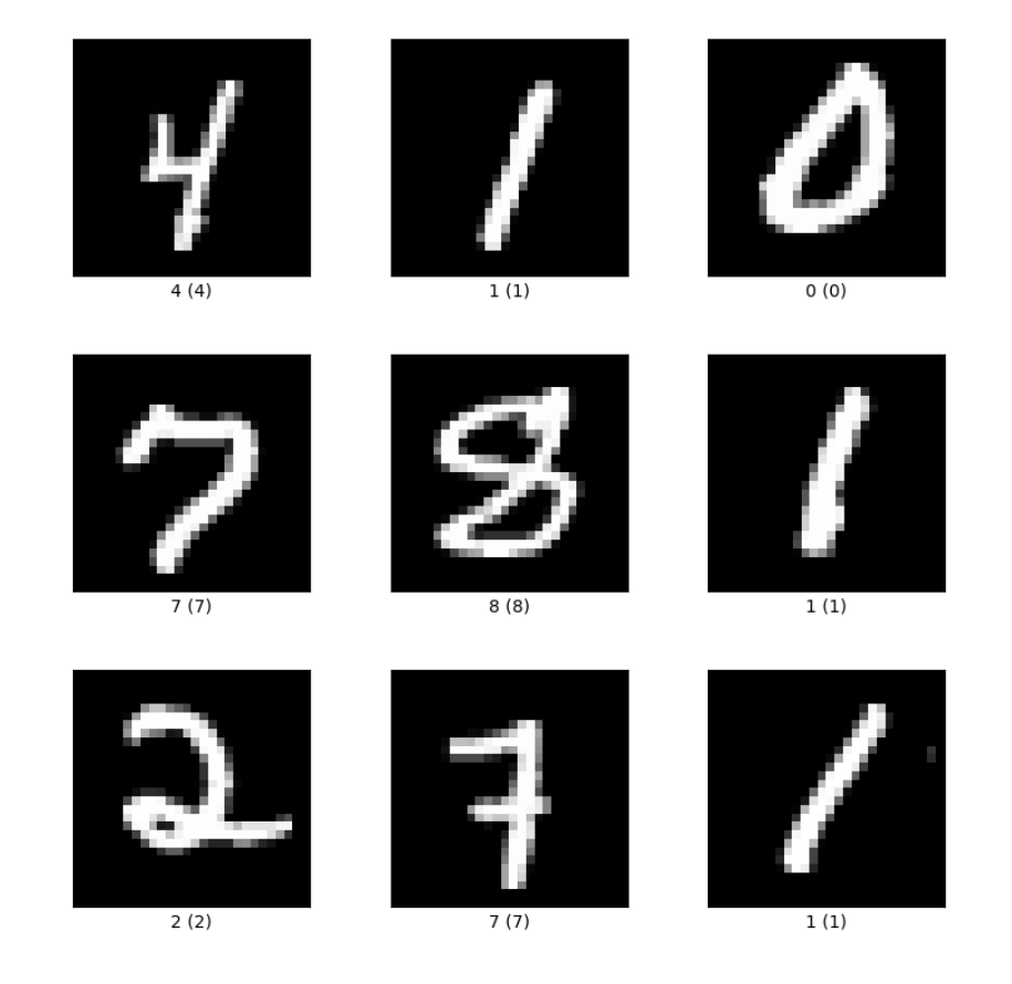
It is always useful to look at your data along the way. Using random.randomint and wandb, we show the label of the image and the image itself from a random index of the training data. Let’s take a look at the first few images in the training set:


Fig 1. A mosaic of handwritten digits and their associated labels from the training dataset.

Building a DNN with torch.Tensor

Let’s start simple and try to build a network that fits x_train to y_train with basic torch components.

We will start with a single layer that uses matrix multiplication and adds a vector of biases. Along with this, we will track the gradients wrt the tensors so will use ‘requires_grad’ in PyTorch.

We create a set of random weights with torch.randn. The size of this weight tensor is (784, 10). The size of an input image in the training set is 784 (images are arrays of 784 entries that have already been flattened, we have 50,000 of them). The weight tensor’s second dimension, 10, corresponds to the number of neurons we have in that layer. We wish to have 10 neurons since we have 10 classes we want to classify (0,1,2,3…9 number of handwritten digit)

We define the linear operation of multiplying an input tensor by the weight tensor and adding the bias as a function. After this, we define a log-softmax operation to normalise the output of the model to return probabilities of each of the 10 classes. We use the log-softmax instead of regular softmax for stability reasons. Also due to its relationship to ‘surprise’ of events happening. When framing the problem as an optimisation problem, we are trying to minimise the surprise of each of the outcomes. Surprise is defined as the negative log of the probability. The expectation of the surprise is the entropy of the system. Cool video here about why we use surprise and why the idea of this optimisation and surprise framing yields the KL-divergence and Maximum Likelihood Estimation. The logarithms of probabilities.

Moving on, we create our model by taking the log softmax of our linear layer of the input batch.

Batching

We use batches to split the training dataset up into smaller chunks. We apply our model to one batch at a time to save throwing everything at it at once.

We achieve this by use of indexing. e.g. x_batch = x_train[0:batch_size]

The output size of the model is equal to the batch size by the dimension of the output neurons. Here the output is a tensor of shape (64, 10). and therefore a dimension of 2.

Loss and metrics

Obviously the output of the current model is rubbish. It’s just the log softmax of random weights multiplied by the input tensor plus a bias of zero. We need a way of quantifying how wrong this output is to inform how to improve it.

Note, all logs are lns (log base e).

We can start by assuming that the output from the model with the highest probability. The log softmax function is defined as $$log(\frac{exp(x_i)}{\sum_{j=1}^n exp(x_j)}) = x_j - log(\sum_{i=1}^n exp (x_i))$$ and this value is negative, so the output with the highest value has the highest predicted probability.

We now define an accuracy metric to find the difference between the highest value outputted by the model and the actual label of the input training sample. We do this by finding the argument of the highest value in the output array and comparing this to the value of the label. (The argument of the output tensor is a single number (0,1,2,3…9) and the argmax will return one of these numbers, i.e. the prediction. We compare that to the actual label, y) The accuracy is then defined as the number of correct predictions divided by the number of total predictions for a batch of inputs.. In this model, the accuracy is around 10% (expected since there are 10 classes and we have random weight initialisation)

Downsides of using argmax

Unfortunately, the argmax function can’t be differentiated, this is pivotal in training neural networks and in particular, they must be smoothly varying. Argmax is no longer an option for us. We can double check this by calling the .backward() function on our accuracy function and see it returns ‘does not have a grad_fn’.

Cross entropy

Instead, we will use a cross-entropy function. Excellent article about cross entropy by Dr. Charles Frye can be seen here. Really recommend this blog post for understanding cross entropy for deep learning.

We use the cross entropy formula to get a new loss function that is differentiable. The expected loss of random guessing on 10 classes is going to be close to $-log(1/10)$. Which it is. 2.31 vs 2.30.

We can now call .backward() on the loss function and PyTorch will smile back at us!

The gradients are stored in the weights.grad, and bias.grad attributes of our model.

Training loop

We now have everything we need:

Data in terms of x_train and y_train
A model with weights and bias
A loss function using cross entropy that we can call .backward on to compute gradients

Let’s create a python for loop that will train the model based on the minimisation of this loss function.

We define two parameters:

Learning rate (i.e. how big of a step in the downwards gradient direction we take)
Epochs (How many times the training data is put through the model)

The for loop is as follows:

lr = 0.5 # learning rate
epochs = 2 # numebr of training epochs

for epoch in range(epochs): # loop over all data
	for ii in range((n-1) // bs + 1): # in batches of size bs, for ~n/bs batches
		start_idx = ii*bs # current array index
		end_idx = start_idx + bs # end batch index

		# Grab the x and y training samples for the current batch
		xb = x_train[start_idx:end_idx]
		yb = y_train[start_idx:end_idx]

		# run the features through the model
		pred = model(xb)

		# calculate the loss
		loss = loss_func(pred, yb)

		# calculate the gradients
		loss.backward()

		# update the model parameters
		with torch.no_grad(): # don't track gradients when updating params
			weights -= weights.grad * lr # update weights by learning rate*grads
			bias -= bias.grad * lr # and for bias
			# delete the current gradients or else they'll compound
			weights.grad.zero()
			bias.grad.zero()

This is the very simple weight and bias update loop for training the model to minimise the loss function for the training features subject to the labels provided.

We then test this on some examples and see if the accuracy of the model has decreased (can use accuracy since this problem has no class imbalances).

Accuracy is now 100%.

Why this training loop is inefficient

We have to write a custom loop every time we write a new model
Lots of hard coded assumptions
Manual tracking of hyper parameters
If we can’t fit data into the ram then we’re done for

Let’s look at torch.nn components to make our lives easier.

First, we don’t need to write our own cross entropy and log softmax from scratch. PyTorch has these built in. It’s less bug prone to use libraries that are already written.

We can find both of these in torch.nn.functional

import torch.nn.functional as F

loss_func = F.cross_entropy

def model(xb):
	return xb @ weights + bias

We can then evaluate the model on a batch with the following:

loss_func(model(xb), yb)
accuracy(model(xb), yb)

which will give us the exact same output as before.

Now, we’re being naïve here, we are defining weights and bias outside of the model function and they are being manipulated all over the place without being tracked. We want to use weights and bias as functions e.g. when making predictions we want to pass them an input and get an output. But weights and bias are stateful (they depend on what has already happened to them and need a current state that may have been updated). They are parameterised functions and can be changed by altering their parameters (through optimisation). We need a way of both calling these items like a function and also tracking their state like an object. Enter nn.Modlue

nn.Module

nn.Module is a PyTorch class that allows us to track state and call as a function. For example

from torch import nn

class MNISTLogistic(nn.Modlue):
	def __init__(self):
		super().__init__() # run parent class init function (nn.Modlue.__init__()
		self.weights = nn.Parameter(torch.randn(784,10)/math.sqrt(784))
		self.biad = nn.Parameter(torch.zeros(10))

This gives us a class that we can call like a function with loss.backward() and instantiate it as an object. We can also add a forward pass function as so:

def forward(self, xb: torch.Tensor)-> torch.Tensor:
	return xb @ weights + bias

and add this to the class with:

MNISTLogistic.forward = forward

We can then instantiate the model as follows:

model = MNISTLogistic() # instantiate like an object
model(xb) # can call like a fn
loss = loss_func(model(xb), yb) # use within other functions
loss.backward() # can still use gradients
model.weights.grad # grads stored in parameter's grad attribute

Even better than all of this is the fact that we can use model.parameters() to iterate over all of the model parameters! Our new training loop will look like this:

def fit():
	for epoch in range(epochs):
		for ii in range((n-1)//bs +1):
			start_idx = ii * bs
			end_idx = start_idx + bs
			xb = x_train[start_ix:end_idx]
			yb = y_train[start_ix:end_idx]
			pred = model(xb)
			loss = loss_func(pred, yb)

			loss.backward()
			with torch.no_grad():
				for p in model.parameters(): # find all model params
					p -= p.grad() * lr # update parameters via SGD
				model.zero_grad() # set gradients to zero to stop accumulation
fit()

We can then calculate the accuracy as before with:

accuracy(model(xb), yb)

But there’s more! torch.nn has so many more modules that we can use. See them all with torch.nn.modules.__all__.

Instead of defining our linear layer, we’ll just use nn.Linear like so:

class MNISTLogistic(nn.Module):
	def __init__(self):
		super.__init__()
		self.lin = nn.Linear(784,10) # already sets up weights and biases
	def forward(self, xb):
		return self.lin(xb) # cals the linear layer

The nn.Linear module is a child of model so we can’t directly see the weight and bias matrices, but we can access them with .parameters

model.children() # returns the Linear layer with in_features=784, out_features = 10 and bias=True
model.parameters() # returns the weight and bias parameters

Gradients

We can calculate the gradients with the torch.optim.Optimizer class like so:

from torch import optim
def configure_optimizer(model: nn.Modlue) -> optim.Optimizer: # returns an optimizer
	return optim.Adam(model.parameters(), lr=3e-4) # Adam optimizer with learning rate of 3e-4

We can then use this optimizer to update the parameters with opt.setp() and opt.zero_grad(). With these functions, we can shorten the training loop further.

Datasets

We’d rather not handle the dataset manually, so let’s abstract some of that away. We can use the torch.utils.data.Dataset class to create a dataset class that we can use to iterate over batches of data. We can then use the torch.utils.data.DataLoader class to create a data loader that we can use to iterate over batches of data.

We use the BaseDataset class as a starting point from the text_recognizer library and create the following:

from text_recognizer.data.util import BaseDataset
train_ds = BaseDataset(X_train, y_train)

Rather than using this and creating our own batches of data, we can use a DataLoader to do this for us. We can create a data loader with:

from torch.utils.data import DataLoader
train_dl = DataLoader(train_ds, batch_size=bs)

We can then define a fit function that uses the data loader to iterate over batches of data and assign it to our model class.

def fit(self: nn.Module, train_dl: DataLoader):
	"""
	Trains the model on the training data using a dataloader
	"""
	opt = configure_optimizer(self)
	for epoch in range(epochs):
		for xb, yb in train_dl:
			pred = model(xb)
			loss = loss_func(pred, yb)

			loss.backward()
			opt.step()
			opt.zero_grad()

MNISTLogistic.fit = fit

After this, it’s super easy to create a model and train it:

model = MNISTLogistic()
model.fit(train_dl)

Super! So much better than what we had before!

What’s even better is we can easily swap out the model for a different model!

We will continue the rest of this lab tomorrow (11/10/2020)! Stay tuned :D <3

Ben Snow

FSDL Lab 1: PyTorch